扩散模型包含两个过程,前向扩散过程(加噪)和反向生成过程(去噪)。前向扩散过程是对一张图像逐渐增加高斯噪声,直至变成图像变为随机噪声;反向生成过程将从一个随机噪声开始逐渐去噪直至生成一张图片,反向去噪过程也即图像生成过程中求解和训练的部分。下图为扩散模型与其他主流生成模型的示意图: 扩散模型与其他主流生成模型

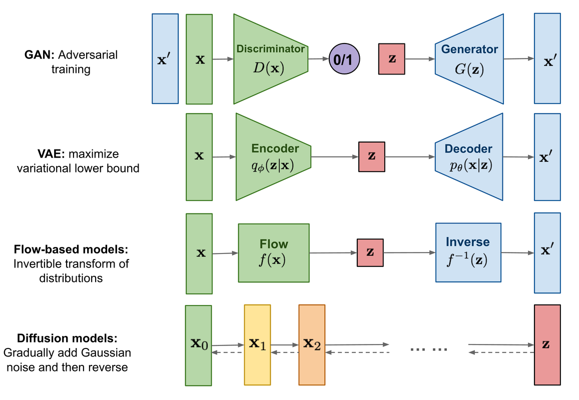
目前所采用的扩散模型大多基于2020年的工作DDPM: Denoising Diffusion Probabilistic Models,其对之前的扩散模型进行了简化(从预测去噪后的图片优化为预测噪声,残差思想),并较大程度上提升了扩散模型的生成效果和稳定性。同时,扩散模型也是一个隐变量模型,可以通过变分推断来进行建模。

扩散模型原理

扩散模型包括两个过程,前向过程(forward process)和反向过程(reverse process),这两个过程都是一个参数化的马尔可夫链(Markov chain)。

前向加噪过程

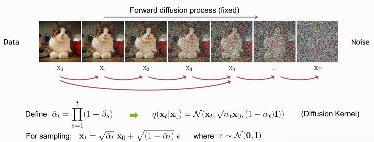
给定一个从原始数据中采样到的真实数据分布 $ x_0 \sim q(x) $,我们定义前向过程为在 T 个步骤内逐渐对数据增加少量高斯噪声,这过程中生成的一系列中间加噪结果记为 $x_1, …, x_T$ 。

前向过程的加噪幅度大小由每一步所采用的方差控制,记为 $\beta_t$ 介于0~1之间,我们通常称不同step对应的方差设定为variance schedule或者noise schedule,通常情况下后靠后的step会采用更大的方差。随着加噪步数的增多 $x_T$ 会逐渐丢失原始数据的特征变为随机噪声,整个扩散过程也可以就是一个马尔可夫链。前向过程可表示为:

$$ q(\mathbf{x}_t|\mathbf{x}_{t-1}) = \mathcal{N}(\mathbf{x}_t; \sqrt{1 - \beta_t}\mathbf{x}_{t-1}, \beta_t\mathbf{I}), q(\mathbf{x}_{1:T}|\mathbf{x}_0) = \prod_{t=1}^T q(\mathbf{x}_t|\mathbf{x}_{t-1}) $$

上述过程一个很好的特性是,根据前向加噪过程和noise schedule,我们可以通过重参数化技巧得到任意时间步下的加噪结果 $ x_T \sim q(x_T | x_0) $,这里定义 $\alpha_t = 1 - \beta_t$ 和 $\bar{\alpha_t} = \prod_{i=1}^t \alpha_i$,那么有:

$$ \begin{aligned} \mathbf{x}_t &= \sqrt{\alpha_t}\mathbf{x}_{t-1} + \sqrt{1 - \alpha_t}\boldsymbol{\epsilon}_{t-1} & \text{ ;where } \boldsymbol{\epsilon}_{t-1}, \boldsymbol{\epsilon}_{t-2}, \dots \sim \mathcal{N}(\mathbf{0}, \mathbf{I}) \\ &= \sqrt{\alpha_t \alpha_{t-1}} \mathbf{x}_{t-2} + \sqrt{1 - \alpha_t \alpha_{t-1}} \bar{\boldsymbol{\epsilon}}_{t-2} & \text{ ;where } \bar{\boldsymbol{\epsilon}}_{t-2} \text{ merges two Gaussians (*).} \\ &= \dots \\ &= \sqrt{\bar{\alpha}_t}\mathbf{x}_0 + \sqrt{1 - \bar{\alpha}_t}\boldsymbol{\epsilon} \end{aligned} $$

上述推到过程利用了两个方差不同的高斯分布 $\mathcal{N}(\mathbf{0},\sigma_1^2\mathbf{I})$ 和 $\mathcal{N}(\mathbf{0},\sigma_2^2\mathbf{I})$ 相加等于一个新的高斯分布。重参数化后可得:

$$ q(\mathbf{x}_t \vert \mathbf{x}_0) = \mathcal{N}(\mathbf{x}_t; \sqrt{\bar{\alpha}_t} \mathbf{x}_0, (1 - \bar{\alpha}_t)\mathbf{I}) $$

扩散过程的这个特性很重要,通过上式我们可以额将 $x_T$ 看作是原始数据$x_0$ 和 随机噪声 $\boldsymbol{\epsilon}$ 的线性组合,其中两者的系数 $\sqrt{\bar{\alpha}_t}$ 和 $\sqrt{1 - \bar{\alpha}_t}$的平方和为1,我们也可以两部分系数为singal rate 和noise rate。通常的在前向加噪过程的 noise schedule中, $\beta_1 < \beta_2 < … < \beta_T$ ,因此 $\bar{\alpha}_1 > \bar{\alpha}_2 > … > \bar{\alpha}_T$。

前向加噪示意图

反向去噪过程

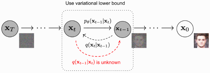
反向过程就是一个去噪的过程,如果我们知道反向过程的每一步的真实分布 $q(x_{t-1} | x_{t})$ ,那么从一个随机噪声 $\mathbf{x_T} \sim \mathcal{N}(\mathbf{0},\mathbf{I})$ 开始,逐渐去噪就能生成一个真实的样本,因此反向过程也就是生成数据的过程。但是我们无法直接去估计 $q({x_{t-1}} | {x_t})$ 的分布(需要用到整个数据集),因此我们通过模型去学习条件概率分布来。

$$ p_\theta(\mathbf{x}_{0:T}) = p(\mathbf{x}_T) \prod^T_{t=1} p_\theta(\mathbf{x}_{t-1} \vert \mathbf{x}_t) \quad p_\theta(\mathbf{x}_{t-1} \vert \mathbf{x}_t) = \mathcal{N}(\mathbf{x}_{t-1}; \boldsymbol{\mu}_\theta(\mathbf{x}_t, t), \boldsymbol{\Sigma}_\theta(\mathbf{x}_t, t)) $$

$p_\theta(\mathbf{x}_{t-1} \vert \mathbf{x}_t)$ 为参数化的高斯分布,它们的均值和方差由训练的网络给出。实际上,扩散模型就是要得到这些训练好的网络,由它们构成了最终的生成模型。

$p_\theta(\mathbf{x}_{t-1} \vert \mathbf{x}_t)$ 是不可直接处理的,但是加上条件 $\mathbf{x}_0$ 的后验分布是可处理的,这里可以将其表示为:

$$ q(\mathbf{x}_{t-1} \vert \mathbf{x}_t, \mathbf{x}_0) = \mathcal{N}(\mathbf{x}_{t-1}; \color{blue}{\tilde{\boldsymbol{\mu}}(\mathbf{x}_t, \mathbf{x}_0)}, \color{red}{\tilde{\beta}_t \mathbf{I}}) $$

首先针对上面的公式,根据贝叶斯公式,可得到:

$$ q(\mathbf{x}_{t-1}|\mathbf{x}_t,\mathbf{x}_0)=q(\mathbf{x}_t|\mathbf{x}_{t-1},\mathbf{x}_0)\frac{q(\mathbf{x}_{t-1}|\mathbf{x}_0)}{q(\mathbf{x}_t|\mathbf{x}_0)} $$

其中由扩散过程的马尔可夫链特性,我们可以得到:

$$ q(\mathbf{x}_t | \mathbf{x}_{t-1}, \mathbf{x}_0) = q(\mathbf{x}_t | \mathbf{x}_{t-1}) = \mathcal{N}(\mathbf{x}_t; \sqrt{1 - \beta_t}\mathbf{x}_{t-1}, \beta_t\mathbf{I}), $$
$$ q(\mathbf{x}_{t-1}|\mathbf{x}_0) = \mathcal{N}\left( \mathbf{x}_{t-1}; \sqrt{\bar{\alpha}_{t-1}}\mathbf{x}_0, (1 - \bar{\alpha}_{t-1})\mathbf{I} \right), q(\mathbf{x}_t|\mathbf{x}_0) = \mathcal{N}\left( \mathbf{x}_t; \sqrt{\bar{\alpha}_t}\mathbf{x}_0, (1 - \bar{\alpha}_t)\mathbf{I} \right) $$
代入上式可得:
$$ \begin{aligned} q(\mathbf{x}_{t-1} \vert \mathbf{x}_t, \mathbf{x}_0) &= q(\mathbf{x}_t \vert \mathbf{x}_{t-1}, \mathbf{x}_0) \frac{ q(\mathbf{x}_{t-1} \vert \mathbf{x}_0) }{ q(\mathbf{x}_t \vert \mathbf{x}_0) } \\ &\propto \exp \Big(-\frac{1}{2} \big(\frac{(\mathbf{x}_t - \sqrt{\alpha_t} \mathbf{x}_{t-1})^2}{\beta_t} + \frac{(\mathbf{x}_{t-1} - \sqrt{\bar{\alpha}_{t-1}} \mathbf{x}_0)^2}{1-\bar{\alpha}_{t-1}} - \frac{(\mathbf{x}_t - \sqrt{\bar{\alpha}_t} \mathbf{x}_0)^2}{1-\bar{\alpha}_t} \big) \Big) \\ &= \exp \Big(-\frac{1}{2} \big(\frac{\mathbf{x}_t^2 - 2\sqrt{\alpha_t} \mathbf{x}_t \color{blue}{\mathbf{x}_{t-1}} \color{black}{+ \alpha_t} \color{red}{\mathbf{x}_{t-1}^2} }{\beta_t} + \frac{ \color{red}{\mathbf{x}_{t-1}^2} \color{black}{- 2 \sqrt{\bar{\alpha}_{t-1}} \mathbf{x}_0} \color{blue}{\mathbf{x}_{t-1}} \color{black}{+ \bar{\alpha}_{t-1} \mathbf{x}_0^2} }{1-\bar{\alpha}_{t-1}} - \frac{(\mathbf{x}_t - \sqrt{\bar{\alpha}_t} \mathbf{x}_0)^2}{1-\bar{\alpha}_t} \big) \Big) \\ &= \exp\Big( -\frac{1}{2} \big( \color{red}{(\frac{\alpha_t}{\beta_t} + \frac{1}{1 - \bar{\alpha}_{t-1}})} \mathbf{x}_{t-1}^2 - \color{blue}{(\frac{2\sqrt{\alpha_t}}{\beta_t} \mathbf{x}_t + \frac{2\sqrt{\bar{\alpha}_{t-1}}}{1 - \bar{\alpha}_{t-1}} \mathbf{x}_0)} \mathbf{x}_{t-1} \color{black}{ + C(\mathbf{x}_t, \mathbf{x}_0) \big) \Big)} \end{aligned} $$

recall:若一个随机变量X服从一个位置参数μ和尺度参数σ的概率分布,且其概率密度函数为: $$ f(x) = \frac{1}{\sqrt{2\pi}\sigma} exp(-\frac{(x - μ)^2}{2σ^2}) $$

这里的 $C(x_t, x_0)$ 是一个和 $x_{t-1}$ 无关的部分,所以省略。根据高斯分布的概率密度函数定义和上述结果(配平方),我们可以得到后验分布 $q(x_{t-1}|x_t, x_0)$ 的均值和方差:

$$ \begin{aligned} \tilde{\beta}_t &= 1/(\frac{\alpha_t}{\beta_t} + \frac{1}{1 - \bar{\alpha}_{t-1}}) = 1/(\frac{\alpha_t - \bar{\alpha}_t + \beta_t}{\beta_t(1 - \bar{\alpha}_{t-1})}) = \color{green}{\frac{1 - \bar{\alpha}_{t-1}}{1 - \bar{\alpha}_t} \cdot \beta_t} \\ \end{aligned} $$
$$ \begin{aligned} \tilde{\boldsymbol{\mu}}_t (\mathbf{x}_t, \mathbf{x}_0) &= (\frac{\sqrt{\alpha_t}}{\beta_t} \mathbf{x}_t + \frac{\sqrt{\bar{\alpha}_{t-1} }}{1 - \bar{\alpha}_{t-1}} \mathbf{x}_0)/(\frac{\alpha_t}{\beta_t} + \frac{1}{1 - \bar{\alpha}_{t-1}}) \\ &= (\frac{\sqrt{\alpha_t}}{\beta_t} \mathbf{x}_t + \frac{\sqrt{\bar{\alpha}_{t-1} }}{1 - \bar{\alpha}_{t-1}} \mathbf{x}_0) \color{green}{\frac{1 - \bar{\alpha}_{t-1}}{1 - \bar{\alpha}_t} \cdot \beta_t} \\ &= \frac{\sqrt{\alpha_t}(1 - \bar{\alpha}_{t-1})}{1 - \bar{\alpha}_t} \mathbf{x}_t + \frac{\sqrt{\bar{\alpha}_{t-1}}\beta_t}{1 - \bar{\alpha}_t} \mathbf{x}_0\\ \end{aligned} $$

通过推到得到的方差和均值的表达式可看出,方式是一个定量(与扩散过程参数有关),均值是依赖 $\mathbf{x}_0$ 和 $\mathbf{x}_t$ 的函数。

优化目标

我们可以将扩散模型中间产生的变量看作隐变量,因此扩散模型可以被视为包含T个隐变量的隐变量模型(latent variable model)。相较于同为隐变量模型的VAE,扩散模型得到的latent是和原始数据同维度的。同时,因为diffusion model可以被视为隐变量模型,我们则可以通过 变分下界(variational lower bound, VLB,又称ELBO) 来优化的负对数似然。具体推导如下:

$$ \begin{aligned} - \log p_\theta(\mathbf{x}_0) &\leq - \log p_\theta(\mathbf{x}_0) + D_\text{KL}(q(\mathbf{x}_{1:T}\vert\mathbf{x}_0) \| p_\theta(\mathbf{x}_{1:T}\vert\mathbf{x}_0) ) \\ &= -\log p_\theta(\mathbf{x}_0) + \mathbb{E}_{\mathbf{x}_{1:T}\sim q(\mathbf{x}_{1:T} \vert \mathbf{x}_0)} \Big[ \log\frac{q(\mathbf{x}_{1:T}\vert\mathbf{x}_0)}{p_\theta(\mathbf{x}_{0:T}) / p_\theta(\mathbf{x}_0)} \Big] \\ &= -\log p_\theta(\mathbf{x}_0) + \mathbb{E}_q \Big[ \log\frac{q(\mathbf{x}_{1:T}\vert\mathbf{x}_0)}{p_\theta(\mathbf{x}_{0:T})} + \log p_\theta(\mathbf{x}_0) \Big] \\ &= \mathbb{E}_q \Big[ \log \frac{q(\mathbf{x}_{1:T}\vert\mathbf{x}_0)}{p_\theta(\mathbf{x}_{0:T})} \Big] \\ \text{Let }L_\text{VLB} &= \mathbb{E}_{q(\mathbf{x}_{0:T})} \Big[ \log \frac{q(\mathbf{x}_{1:T}\vert\mathbf{x}_0)}{p_\theta(\mathbf{x}_{0:T})} \Big] \end{aligned} $$

我们进一步对目标函数进行分解:

$$ \begin{aligned} L_\text{VLB} &= \mathbb{E}_{q(\mathbf{x}_{0:T})} \Big[ \log\frac{q(\mathbf{x}_{1:T}\vert\mathbf{x}_0)}{p_\theta(\mathbf{x}_{0:T})} \Big] \\ &= \mathbb{E}_q \Big[ \log\frac{\prod_{t=1}^T q(\mathbf{x}_t\vert\mathbf{x}_{t-1})}{ p_\theta(\mathbf{x}_T) \prod_{t=1}^T p_\theta(\mathbf{x}_{t-1} \vert\mathbf{x}_t) } \Big] \\ &= \mathbb{E}_q \Big[ -\log p_\theta(\mathbf{x}_T) + \sum_{t=1}^T \log \frac{q(\mathbf{x}_t\vert\mathbf{x}_{t-1})}{p_\theta(\mathbf{x}_{t-1} \vert\mathbf{x}_t)} \Big] \\ &= \mathbb{E}_q \Big[ -\log p_\theta(\mathbf{x}_T) + \sum_{t=2}^T \log \frac{q(\mathbf{x}_t\vert\mathbf{x}_{t-1})}{p_\theta(\mathbf{x}_{t-1} \vert\mathbf{x}_t)} + \log\frac{q(\mathbf{x}_1 \vert \mathbf{x}_0)}{p_\theta(\mathbf{x}_0 \vert \mathbf{x}_1)} \Big] \\ &= \mathbb{E}_q \Big[ -\log p_\theta(\mathbf{x}_T) + \sum_{t=2}^T \log \Big( \frac{q(\mathbf{x}_{t-1} \vert \mathbf{x}_t, \mathbf{x}_0)}{p_\theta(\mathbf{x}_{t-1} \vert\mathbf{x}_t)}\cdot \frac{q(\mathbf{x}_t \vert \mathbf{x}_0)}{q(\mathbf{x}_{t-1}\vert\mathbf{x}_0)} \Big) + \log \frac{q(\mathbf{x}_1 \vert \mathbf{x}_0)}{p_\theta(\mathbf{x}_0 \vert \mathbf{x}_1)} \Big] \\ &= \mathbb{E}_q \Big[ -\log p_\theta(\mathbf{x}_T) + \sum_{t=2}^T \log \frac{q(\mathbf{x}_{t-1} \vert \mathbf{x}_t, \mathbf{x}_0)}{p_\theta(\mathbf{x}_{t-1} \vert\mathbf{x}_t)} + \sum_{t=2}^T \log \frac{q(\mathbf{x}_t \vert \mathbf{x}_0)}{q(\mathbf{x}_{t-1} \vert \mathbf{x}_0)} + \log\frac{q(\mathbf{x}_1 \vert \mathbf{x}_0)}{p_\theta(\mathbf{x}_0 \vert \mathbf{x}_1)} \Big] \\ &= \mathbb{E}_q \Big[ -\log p_\theta(\mathbf{x}_T) + \sum_{t=2}^T \log \frac{q(\mathbf{x}_{t-1} \vert \mathbf{x}_t, \mathbf{x}_0)}{p_\theta(\mathbf{x}_{t-1} \vert\mathbf{x}_t)} + \log\frac{q(\mathbf{x}_T \vert \mathbf{x}_0)}{q(\mathbf{x}_1 \vert \mathbf{x}_0)} + \log \frac{q(\mathbf{x}_1 \vert \mathbf{x}_0)}{p_\theta(\mathbf{x}_0 \vert \mathbf{x}_1)} \Big]\\ &= \mathbb{E}_q \Big[ \log\frac{q(\mathbf{x}_T \vert \mathbf{x}_0)}{p_\theta(\mathbf{x}_T)} + \sum_{t=2}^T \log \frac{q(\mathbf{x}_{t-1} \vert \mathbf{x}_t, \mathbf{x}_0)}{p_\theta(\mathbf{x}_{t-1} \vert\mathbf{x}_t)} - \log p_\theta(\mathbf{x}_0 \vert \mathbf{x}_1) \Big] \\ &= \mathbb{E}_q [\underbrace{D_\text{KL}(q(\mathbf{x}_T \vert \mathbf{x}_0) \parallel p_\theta(\mathbf{x}_T))}_{L_T} + \sum_{t=2}^T \underbrace{D_\text{KL}(q(\mathbf{x}_{t-1} \vert \mathbf{x}_t, \mathbf{x}_0) \parallel p_\theta(\mathbf{x}_{t-1} \vert\mathbf{x}_t))}_{L_{t-1}} \underbrace{- \log p_\theta(\mathbf{x}_0 \vert \mathbf{x}_1)}_{L_0} ] \end{aligned} $$

反向去噪过程示意图: diffusion模型优化目标示意图

从上面推导出的目标函数中可以看到,其一共包含T+1项,其中 $L_0$ 可以看成是原始数据重建,优化的是负对数似然,可以用估计的 $\mathcal{N}(x_0;\mu_\theta(x_1, 1), \Sigma_\theta(x_1, 1))$ 来构建一个离散化的 decoder 来计算。$L_T$ 计算的是最后得到的噪声的分布和先验分布(高斯噪声)间的KL散度,这个KL散度没有训练参数,且我们的前向过程可以实现这一点,因此可以近似为0。由此我们的优化目标可以focus在 $L_{t-1}$ 上, $L_{t-1}$ 计算的是估计分布 $p_\theta(x_{t-1} \mid x_t)$ 和真实后验分布 $q(x_{t-1} \mid x_t, x_0)$ 之间的 KL 散度,这里我们可以理解为训练目标为使得估计的去噪过程和依赖真实数据的去噪过程近似一致。

$L_{t-1}$ 表示的两个分布间的优化可视为: diffusion模型优化目标示意图

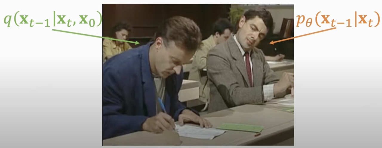
进一步的对于 $L_{t-1}$ 项,之所以前面我们将 $p_\theta(x_{t-1}|x_t)$ 定义为一个用网络参数化的高斯分布 $\mathcal{N}(x_{t-1}; \mu_\theta(x_t, t), \Sigma_\theta(x_t, t))$,是因为要匹配的后验分布 $q(x_{t-1}|x_t, x_0)$ 也是高斯分布,希望得到训练好的网络 $\mu_\theta(x_t, t)$ 和 $\Sigma_\theta(x_t, t)$。

recall:上述反向过程推到得出:

$$ \tilde{\beta}_t = \frac{1 - \bar{\alpha}_{t-1}}{1 - \bar{\alpha}_t} \cdot \beta_t, $$ $$ \tilde{\boldsymbol{\mu}}_t (\mathbf{x}_t, \mathbf{x}_0) = \frac{\sqrt{\alpha_t}(1 - \bar{\alpha}_{t-1})}{1 - \bar{\alpha}_t} \mathbf{x}_t + \frac{\sqrt{\bar{\alpha}_{t-1}}\beta_t}{1 - \bar{\alpha}_t} \mathbf{x}_0 $$ $$ \mathbf{x}_0 = -\frac{1}{\sqrt{\bar{\alpha}_t}} (\mathbf{x}_t - \sqrt{1-\bar{\alpha}_t} \epsilon_t) $$

DDPM对$p_\theta(x_{t-1}|x_t)$做了进一步简化,采用固定的方差:$\Sigma_\theta(x_t, t)=\sigma_t^2 I$,这里的$\sigma_t^2$可以设定为$\beta_t$或者$\tilde{\beta}_t$(这其实是两个极端,分别是上限和下限,这里的方差也可以采用可训练的方差(如IDDPM)。这里我们设定 $\sigma_t^2 = \tilde{\beta}_t$。

$$ q(\mathbf{x}_{t-1}|\mathbf{x}_t, \mathbf{x}_0) = \mathcal{N}\left( \mathbf{x}_{t-1}; \tilde{\mu}(\mathbf{x}_t, \mathbf{x}_0), \sigma_t^2\mathbf{I} \right), $$ $$ p_\theta(\mathbf{x}_{t-1}|\mathbf{x}_t) = \mathcal{N}\left( \mathbf{x}_{t-1}; \mu_\theta(\mathbf{x}_t, t), \sigma_t^2\mathbf{I} \right) $$

对于均值项,我们可以进一步推导,希望训练的 $\mu_\theta$ ,能够预测 $\tilde{\mu_t} = \frac{1}{\sqrt{\bar{\alpha}_t}}\left( \mathbf{x}_t - \frac{1-\bar{\alpha}_t}{\sqrt{1-\bar{\alpha}_t}}\epsilon_t \right)$ ,见下式:

$$ \begin{aligned} \tilde{\mu}_t &= \frac{\sqrt{\bar{\alpha}_t}(1-\bar{\alpha}_{t-1})}{1-\bar{\alpha}_t}\mathbf{x}_t + \frac{\sqrt{\bar{\alpha}_t-1}\beta_t}{1-\bar{\alpha}_t}\frac{1}{\sqrt{\bar{\alpha}_t}}(\mathbf{x}_t - \sqrt{1-\bar{\alpha}_t}\epsilon_t) \\ &= \frac{1}{\sqrt{\bar{\alpha}_t}}\left( \mathbf{x}_t - \frac{1-\bar{\alpha}_t}{\sqrt{1-\bar{\alpha}_t}}\epsilon_t \right) \end{aligned} $$

同时由于 $\mathbf{x_t}$ 在训练时是已知项无需预测,所以我们可以进一步简化 $\mu_\theta$ ,使网络直接预测 $\mathbf{x_t}$ 输入在时间步t下的噪声:

$$ \begin{equation} \mu_{\theta}(\mathbf{x}_t, t) = \frac{1}{\sqrt{\alpha_t}} \left( \mathbf{x}_t - \frac{1-\alpha_t}{\sqrt{1-\bar{\alpha}_t}} \epsilon_{\theta}(\mathbf{x}_t, t) \right) \end{equation} $$
$$ \text{Thus } \mathbf{x}_{t-1} = \mathcal{N}\left(\mathbf{x}_{t-1}; \frac{1}{\sqrt{\alpha_t}} \left( \mathbf{x}_t - \frac{1-\alpha_t}{\sqrt{1-\bar{\alpha}_t}} \epsilon_{\theta}(\mathbf{x}_t, t) \right), \sigma_t^2\mathbf{I} \right) $$

因此 $L_{t-1}$ 项被重参数化为直接最小化 $\tilde\mu$ 和 $\mu_{\theta}$ 见的差异,也即直接最小化 $\epsilon_t$ 和 $\epsilon_{\theta}$ 之间的差异:

$$ \begin{aligned} L_t &= \mathbb{E}_{\mathbf{x}_0, \epsilon} \left[ \frac{1}{2 \| \Sigma_\theta(\mathbf{x}_t, t) \|_2^2} \| \hat{\mu}_t(\mathbf{x}_t, \mathbf{x}_0) - \mu_\theta(\mathbf{x}_t, t) \|_2^2 \right] \\ &= \mathbb{E}_{\mathbf{x}_0, \epsilon} \left[ \frac{1}{2 \| \Sigma_\theta \|_2^2} \frac{1}{\sqrt{\alpha_t}} \left( \mathbf{x}_t - \frac{1 - \alpha_t}{\sqrt{1 - \bar{\alpha}_t}} \epsilon_t \right) - \frac{1}{\sqrt{\alpha_t}} \left( \mathbf{x}_t - \frac{1 - \alpha_t}{\sqrt{1 - \bar{\alpha}_t}} \epsilon_\theta(\mathbf{x}_t, t) \right) \|_2^2 \right] \\ &= \mathbb{E}_{\mathbf{x}_0, \epsilon} \left[ \frac{(1 - \alpha_t)^2}{2 \alpha_t (1 - \bar{\alpha}_t) \| \Sigma_\theta \|_2^2} \| \epsilon_t - \epsilon_\theta(\mathbf{x}_t, t) \|_2^2 \right] \\ &= \mathbb{E}_{\mathbf{x}_0, \epsilon} \left[ \frac{(1 - \alpha_t)^2}{2 \alpha_t (1 - \bar{\alpha}_t) \| \Sigma_\theta \|_2^2} \| \epsilon_t - \epsilon_\theta(\sqrt{\bar{\alpha}_t} \mathbf{x}_0 + \sqrt{1 - \bar{\alpha}_t} \epsilon_t, t) \|_2^2 \right] \end{aligned} $$

进一步,我们可以将损失简化为:

$$ \begin{aligned} L_t^{\text{simple}} &= \mathbb{E}_{t \sim [1, T], \mathbf{x}_0, \epsilon_t} \left[ \| \epsilon_t - \epsilon_\theta(\mathbf{x}_t, t) \|^2 \right] \\ &= \mathbb{E}_{t \sim [1, T], \mathbf{x}_0, \epsilon_t} \left[ \| \epsilon_t - \epsilon_\theta( \sqrt{\bar{\alpha}_t} \mathbf{x}_0 + \sqrt{1-\bar{\alpha}_t} \epsilon_t , t ) \|^2 \right] \end{aligned} $$

最终我们得到的优化目标非常简单,即让网络预测的噪音和真实的噪音一致。

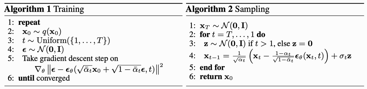
训练过程:DDPM的训练过程也非常简单,如下面的算法流程图所示:随机选择一个训练样本从1-T随机抽样一个t -> 随机产生噪音-计算当前所产生的带噪音数据 -> 输入网络预测噪音 -> 计算产生的噪音和预测的噪音的L2损失 -> 计算梯度并更新网络。

采样过程:DDPM的采样过程如下面的算法流程图所示:从一个随机噪音开始,用训练好的网络预测噪音,然后计算条件分布的均值,然后用均值乘标准差再加以一个随机噪音,直至t=0完成新样本的生成(最后一次迭代不加噪声)。

DDPM 训练、采样 算法流程: 训练、采样 算法流程

DDPM 加噪、采样、训练代码实现:

  1# beta schedule
  2def linear_beta_schedule(timesteps):
  3    scale = 1000 / timesteps
  4    beta_start = scale * 0.0001
  5    beta_end = scale * 0.02
  6    return torch.linspace(beta_start, beta_end, timesteps, dtype=torch.float64)
  7
  8class GaussianDiffusion:
  9    def __init__(
 10        self,
 11        timesteps=1000,
 12        beta_schedule='linear'
 13    ):
 14        self.timesteps = timesteps
 15        
 16        if beta_schedule == 'linear':
 17            betas = linear_beta_schedule(timesteps)
 18        elif beta_schedule == 'cosine':
 19            betas = cosine_beta_schedule(timesteps)
 20        else:
 21            raise ValueError(f'unknown beta schedule {beta_schedule}')
 22        self.betas = betas
 23            
 24        self.alphas = 1. - self.betas
 25        self.alphas_cumprod = torch.cumprod(self.alphas, axis=0)
 26        self.alphas_cumprod_prev = F.pad(self.alphas_cumprod[:-1], (1, 0), value=1.)
 27        
 28        # calculations for diffusion q(x_t | x_{t-1}) and others
 29        self.sqrt_alphas_cumprod = torch.sqrt(self.alphas_cumprod)
 30        self.sqrt_one_minus_alphas_cumprod = torch.sqrt(1.0 - self.alphas_cumprod)
 31        self.log_one_minus_alphas_cumprod = torch.log(1.0 - self.alphas_cumprod)
 32        self.sqrt_recip_alphas_cumprod = torch.sqrt(1.0 / self.alphas_cumprod)
 33        self.sqrt_recipm1_alphas_cumprod = torch.sqrt(1.0 / self.alphas_cumprod - 1)
 34        
 35        # calculations for posterior q(x_{t-1} | x_t, x_0)
 36        self.posterior_variance = (
 37            self.betas * (1.0 - self.alphas_cumprod_prev) / (1.0 - self.alphas_cumprod)
 38        )
 39        # below: log calculation clipped because the posterior variance is 0 at the beginning
 40        # of the diffusion chain
 41        self.posterior_log_variance_clipped = torch.log(self.posterior_variance.clamp(min =1e-20))
 42        
 43        self.posterior_mean_coef1 = (
 44            self.betas * torch.sqrt(self.alphas_cumprod_prev) / (1.0 - self.alphas_cumprod)
 45        )
 46        self.posterior_mean_coef2 = (
 47            (1.0 - self.alphas_cumprod_prev)
 48            * torch.sqrt(self.alphas)
 49            / (1.0 - self.alphas_cumprod)
 50        )
 51    
 52    # get the param of given timestep t
 53    def _extract(self, a, t, x_shape):
 54        batch_size = t.shape[0]
 55        out = a.to(t.device).gather(0, t).float()
 56        out = out.reshape(batch_size, *((1,) * (len(x_shape) - 1)))
 57        return out
 58    
 59    # forward diffusion get x_t from x_0 (using the nice property): q(x_t | x_0)
 60    def q_sample(self, x_start, t, noise=None):
 61        if noise is None:
 62            noise = torch.randn_like(x_start)
 63
 64        sqrt_alphas_cumprod_t = self._extract(self.sqrt_alphas_cumprod, t, x_start.shape)
 65        sqrt_one_minus_alphas_cumprod_t = self._extract(self.sqrt_one_minus_alphas_cumprod, t, x_start.shape)
 66
 67        return sqrt_alphas_cumprod_t * x_start + sqrt_one_minus_alphas_cumprod_t * noise
 68    
 69    # Get the mean and variance of q(x_t | x_0).
 70    def q_mean_variance(self, x_start, t):
 71        mean = self._extract(self.sqrt_alphas_cumprod, t, x_start.shape) * x_start
 72        variance = self._extract(1.0 - self.alphas_cumprod, t, x_start.shape)
 73        log_variance = self._extract(self.log_one_minus_alphas_cumprod, t, x_start.shape)
 74        return mean, variance, log_variance
 75    
 76    # Compute the mean and variance of the diffusion posterior: q(x_{t-1} | x_t, x_0)
 77    def q_posterior_mean_variance(self, x_start, x_t, t):
 78        posterior_mean = (
 79            self._extract(self.posterior_mean_coef1, t, x_t.shape) * x_start
 80            + self._extract(self.posterior_mean_coef2, t, x_t.shape) * x_t
 81        )
 82        posterior_variance = self._extract(self.posterior_variance, t, x_t.shape)
 83        posterior_log_variance_clipped = self._extract(self.posterior_log_variance_clipped, t, x_t.shape)
 84        return posterior_mean, posterior_variance, posterior_log_variance_clipped
 85    
 86    # compute x_0 from x_t and pred noise: the reverse of `q_sample`
 87    def predict_start_from_noise(self, x_t, t, noise):
 88        return (
 89            self._extract(self.sqrt_recip_alphas_cumprod, t, x_t.shape) * x_t -
 90            self._extract(self.sqrt_recipm1_alphas_cumprod, t, x_t.shape) * noise
 91        )
 92    
 93    # compute predicted mean and variance of p(x_{t-1} | x_t)
 94    def p_mean_variance(self, model, x_t, t, clip_denoised=True):
 95        # predict noise using model
 96        pred_noise = model(x_t, t)
 97        # get the predicted x_0: different from the algorithm2 in the paper
 98        x_recon = self.predict_start_from_noise(x_t, t, pred_noise)
 99        if clip_denoised:
100            x_recon = torch.clamp(x_recon, min=-1., max=1.)
101        model_mean, posterior_variance, posterior_log_variance = \
102                    self.q_posterior_mean_variance(x_recon, x_t, t)
103        return model_mean, posterior_variance, posterior_log_variance
104        
105    # denoise_step: sample x_{t-1} from x_t and pred_noise
106    @torch.no_grad()
107    def p_sample(self, model, x_t, t, clip_denoised=True):
108        # predict mean and variance
109        model_mean, _, model_log_variance = self.p_mean_variance(model, x_t, t,
110                                                    clip_denoised=clip_denoised)
111        noise = torch.randn_like(x_t)
112        # no noise when t == 0
113        nonzero_mask = ((t != 0).float().view(-1, *([1] * (len(x_t.shape) - 1))))
114        # compute x_{t-1}
115        pred_img = model_mean + nonzero_mask * (0.5 * model_log_variance).exp() * noise
116        return pred_img
117    
118    # denoise: reverse diffusion
119    @torch.no_grad()
120    def p_sample_loop(self, model, shape):
121        batch_size = shape[0]
122        device = next(model.parameters()).device
123        # start from pure noise (for each example in the batch)
124        img = torch.randn(shape, device=device)
125        imgs = []
126        for i in tqdm(reversed(range(0, timesteps)), desc='sampling loop time step', total=timesteps):
127            img = self.p_sample(model, img, torch.full((batch_size,), i, device=device, dtype=torch.long))
128            imgs.append(img.cpu().numpy())
129        return imgs
130    
131    # sample new images
132    @torch.no_grad()
133    def sample(self, model, image_size, batch_size=8, channels=3):
134        return self.p_sample_loop(model, shape=(batch_size, channels, image_size, image_size))
135    
136    # compute train losses
137    def train_losses(self, model, x_start, t):
138        # generate random noise
139        noise = torch.randn_like(x_start)
140        # get x_t
141        x_noisy = self.q_sample(x_start, t, noise=noise)
142        predicted_noise = model(x_noisy, t)
143        loss = F.mse_loss(noise, predicted_noise)
144        return loss

其中:

q_sample 为整个前向过程,实现从 $x_0$ 到 $x_t$ 的加噪过程;

p_sample_loop 为整个反向去噪过程,实现从 $x_t$ 到 $x_0$ 的去噪过程,也即生成过程;

p_sample 为p_sample_loop中单步的去噪过程,实现从 $x_t$ 通过预测的均值乘标准差加一个随机噪声,得到 $x_{t-1}$ 的过程;

p_mean_variance 为根据预测的噪声,来计算 $p(x_{t-1} | x_t)$ 的均值和方差;

predict_start_from_noise 为q_sample的逆过程,根据预测的噪音来生成 $x_0$ ;

q_posterior_mean_variance 为后验分布 $q(x_{t-1} | x_t, x_0)$ 中均值和方差的计算。